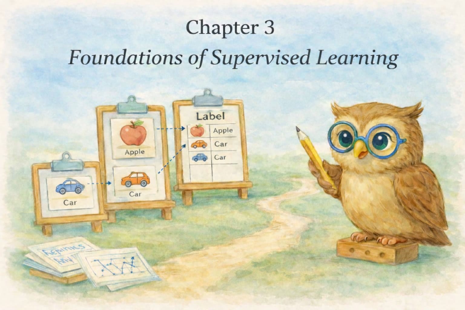
Foundations of Supervised Learning

What Supervised Learning Really Means

In Chapter 2, Tensor Owl shared the basic idea of how machines reason, inspired by human thinking. To reason well, machines must first learn. One of the ways they learn is through supervised learning.

Initially, Tensor Owl had a different understanding of what supervised learning meant. He assumed that a program makes a prediction, and another algorithm supervises whether it is correct. Over time, he realised that supervision comes from the data itself.
Now, when he thinks of supervised learning, he remembers his childhood. In a classroom, the teacher would hold up a picture of an apple and say its name. Then she would hold up a picture of an orange and name it.

After many such examples, he no longer needed guidance. When shown a new picture of the same fruits, different from the ones he had seen before, he could identify them correctly.

Similarly, in supervised learning, training data contains features (inputs) along with their corresponding output. These are provided together for every example. During training, the model learns patterns from the features and predicts an output. This prediction is then compared with the known output present in the training data.

The term supervised comes from the presence of these known outputs in the data. They act as a reference during learning. The model does not receive guidance from a person or another algorithm, but from the answers already provided in the dataset.

Classification vs Regression

Tensor Owl had always been curious about the algorithms used in machine learning. He studied them during his Master’s, but never had the opportunity to apply them in real-world projects.

These algorithms are designed to solve specific types of problems. In supervised machine learning, these problems can be broadly categorized into two main types: Classification and Regression.

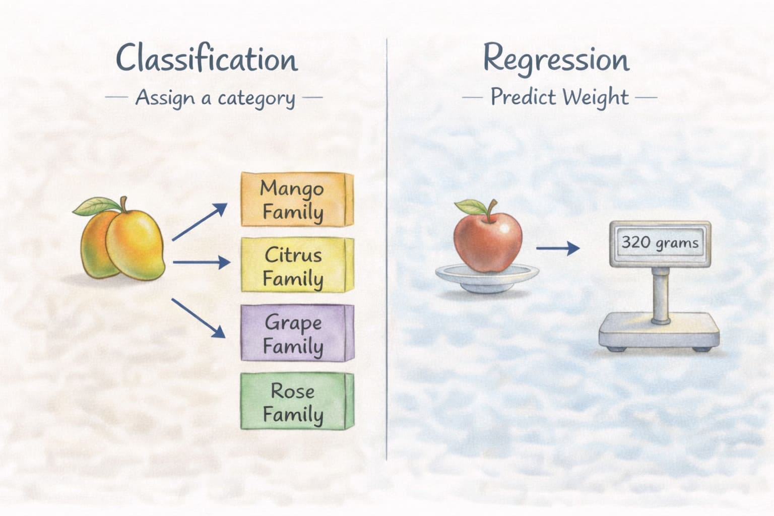
Classification

A classification algorithm predicts the category or label to which an input belongs. The model looks at the input features and maps them to one of the predefined categories.
For example, given an image of a fruit, the model can predict which fruit family it belongs to. Given an email, the model can predict whether it is spam or not.

The possible outputs are already defined. The algorithm simply decides which category best matches the input.

How Does a Classification Model Decide?

You might also be curious, like Tensor Owl, “how a model decides the category?” During training, the model is shown many inputs along with their correct labels. Over time, it begins to notice patterns.
For example, when a model is trained to detect spam emails, it is given normal as well as spam emails. Training data with spam emails contains words like offer, lottery, free, or win.

So when this model is deployed, it reads the content of the email and applies its past learning. The model does not understand the meaning like a human. It only recognises patterns in the data. When a new email arrives, it checks the features, compares them with what it has learned, and predicts the most likely category.

Regression

A regression algorithm predicts a numerical value. The model looks at the input features and estimates a value based on learned patterns.
For example, given the size of a fruit, the model can predict the weight of the fruit. Given cricket match statistics, it can predict the expected score after a certain number of overs. In both cases, the output is a number. Unlike classification, where the result is a category, regression produces a value that can vary within a range.

How Does a Regression Model Decide?

Let’s consider a food delivery platform. Suppose we have past delivery records like this with input features: distance, Traffic, and order size:

Distance (km)	Traffic Level	Order Size	Delivery Time (minutes)
2	Low	Small	18
5	High	Medium	40
3	Medium	Small	25
8	High	Large	55
4	Medium	Medium	30
6	High	Medium	?

If Tensor Owl asks what the approximate delivery time for the 6th case is, you naturally start comparing it with similar rows. Row 2 has High traffic and Medium order size, just like the 6th row. Its delivery time is 40 minutes, but the distance is 5 km. In the 6th row, the distance is 6 km, which is slightly higher. Looking at other rows, we can see that as the distance increases, the delivery time also increases. So it is reasonable to expect the delivery time to be slightly more than 40 minutes. Based on the data pattern, the estimate might be around 42–45 minutes.

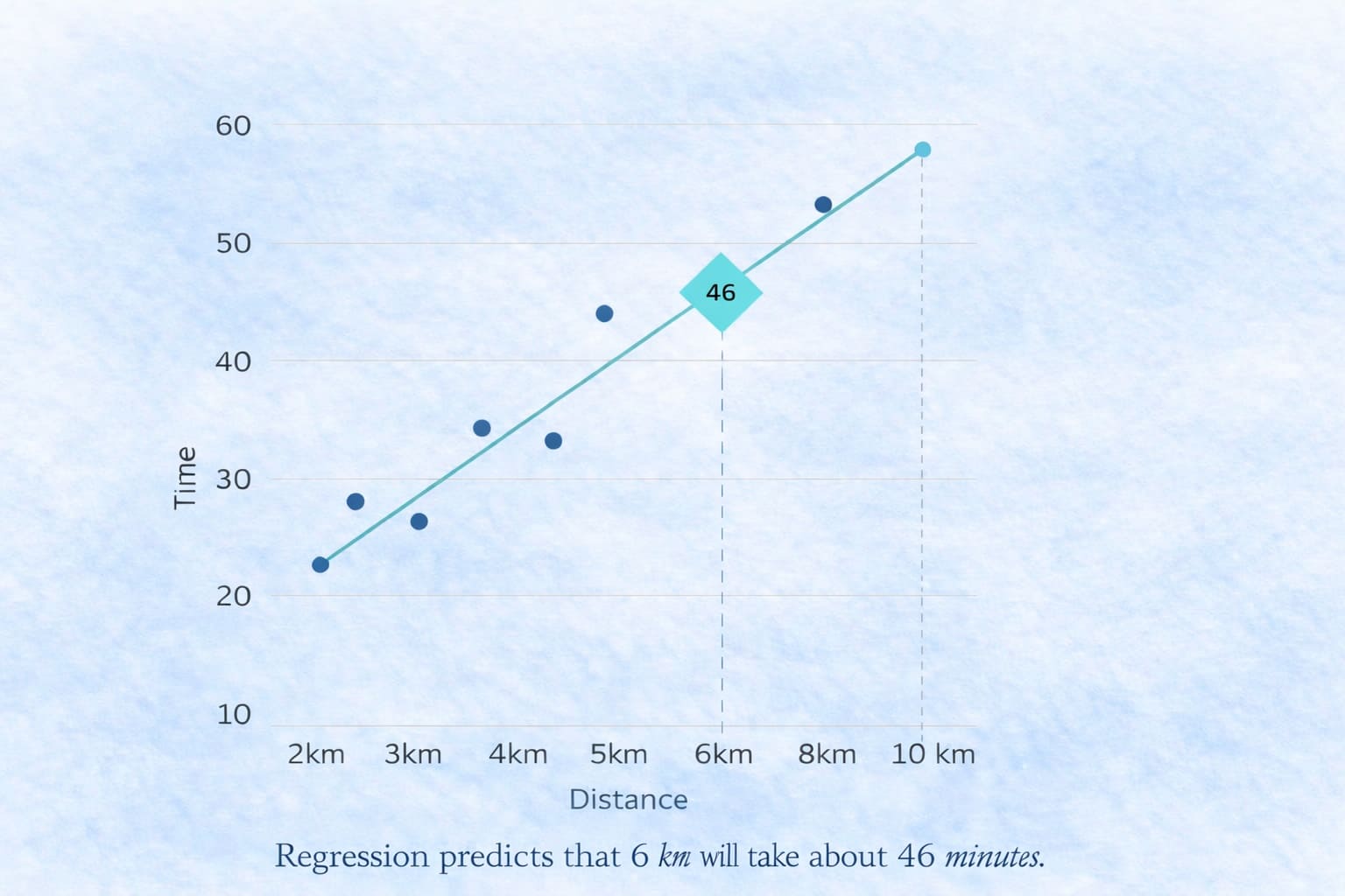
This is exactly what a regression model does. The model does not understand the meaning of traffic or order size. It only learns patterns between input features and numbers. When a new input is given, it uses those learned patterns to estimate a value. In simple terms: A regression model tries to find the best-fitting line (or curve) through the data.

Imagine plotting:
- Distance on the x-axis.
- Delivery Time on the y-axis.

A linear regression model finds the line that best fits all points, and then uses that line to estimate the delivery time for the 6 km case by reading the value where 6 intersects the line.

Dataset Anatomy

A supervised learning model requires structured data. A simple tabular dataset arranged in rows and columns.

This structured table has a few essential properties:

Features:

These are the input columns in the table. They describe the situation or observation captured in the data. Features can be of different types: - Numerical: Distance, Price, Age - Categorical: Traffic Level (Low, Medium, High) - Ordinal: Order Size (Small, Medium, Large) Categorical values are converted into numerical form before training.

Label:

This is the output column. It contains the value the model must learn to predict. For example, Delivery Time is the label.

Samples:

These are the rows in the table. Each row represents one recorded experience. It contains both the input features and the corresponding label.

Splitting the Dataset

After preparing the dataset, it is divided into two parts:

Training set:

This part is used for learning. The model reads the features, makes predictions, compares them with the known labels, and gradually adjusts itself.

Testing set:

This part is kept separate and is not used during learning. It is used only after training to evaluate how well the model performs on unseen data.

This separation ensures that the evaluation reflects real prediction, not memorisation of the training data.

Learning as Optimisation

In Chapter 2, Tensor Owl explained that machine learning is not about memorisation — it is about optimisation.

Supervised learning follows the same principle.
At its core, supervised learning is a structured optimisation problem. A model makes predictions, a loss function measures how wrong those predictions are, and an optimisation algorithm adjusts the parameters to reduce that error.

In supervised learning, the model is expressed as a hypothesis function that maps inputs to predicted outputs.

Hypothesis Function

y^=hθ(x)

x — Input Features: The input values given to the model.
For example, in a food delivery time prediction system, features include distance to the destination, current traffic level, and order size.

θ — Model Parameters: The internal values of the model that determine how strongly each feature influences the prediction.
For example, the model may learn how traffic and distance affect delivery time.

hθ — Hypothesis Function: The mathematical function that combines the input features and model parameters to produce a prediction.
For example, the function may combine distance and traffic data using learned parameters to estimate delivery time.

ŷ — Predicted Output: The value predicted by the model for a given input.
For example, given the distance and current traffic, the model predicts the delivery time.

Once the model makes a prediction, it may not be perfectly correct. As discussed in Chapter 2 by Tensor Owl, predictions always carry some degree of error.

For example, the model may predict that a delivery will take 28 minutes, while the actual delivery time turns out to be 32 minutes.

To improve the model, we must measure how wrong the prediction is. This is where the loss function comes in.

Loss Function (Measuring Error)

A loss function quantifies how far the prediction is from the actual value. This error is expressed using a mathematical function.

Loss Function

L(y, ŷ)

y — True Output: The actual value observed in the dataset.
For example, the real delivery time is recorded after the order is completed.

L(y, ŷ) — Loss Function: A function that measures the difference between the true value and the predicted value. This value represents how wrong the model’s prediction was.

The loss function helps improve the model by measuring how wrong its predictions are and guiding the optimisation process to reduce that error. However, even after minimising the loss, a model can still make mistakes in its predictions.

These errors usually arise for two fundamental reasons. Sometimes the model is too simple, so it cannot capture the real patterns in the data. Other times, the model becomes too complex and starts learning noise instead of the true signal.
This is similar to how humans make mistakes. Sometimes our understanding is too shallow, so we miss important details. Other times, we overthink things and see patterns that are not really there.

Bias, Variance & the Trade-off

Errors in a model’s predictions can arise from different sources. In machine learning, these errors are broadly categorised into two types based on their source: bias and variance.

Bias: Error that occurs when the model is too simple to capture the true patterns in the data. It makes strong assumptions about how the data behaves and therefore misses important relationships.
For example, if we predict delivery time using only distance while ignoring traffic conditions, the model may consistently make similar mistakes because it lacks enough flexibility to represent the real-world situation.

Variance: Error that occurs when the model becomes too sensitive to the training data. Instead of learning the general pattern, it begins to capture small fluctuations or noise in the data.
For example, if the model tries to learn delivery time by closely fitting every past delivery record—including unusual delays caused by accidents or temporary road closures—it may start predicting longer delivery times even when traffic conditions are normal.

A good model finds a balance between these two sources of error. This balance is known as the Bias–Variance Trade-off.

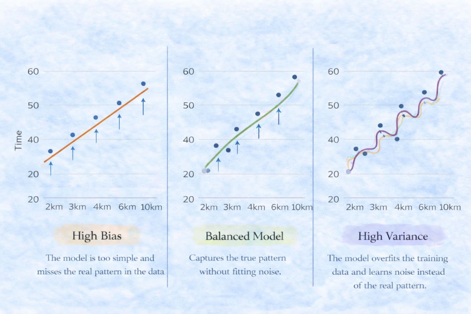
If you observe the high bias case, the model assumes a simple linear relationship between distance and delivery time. Because the model is too simple, it fails to capture the true pattern in the data and consistently makes prediction errors.

A balanced model captures the overall trend in the data and produces reliable predictions without fitting noise.

In contrast, a high-variance model tries to fit almost every point in the training data. As a result, it begins to learn noise and small fluctuations instead of the true underlying pattern, leading to unstable predictions on new data.

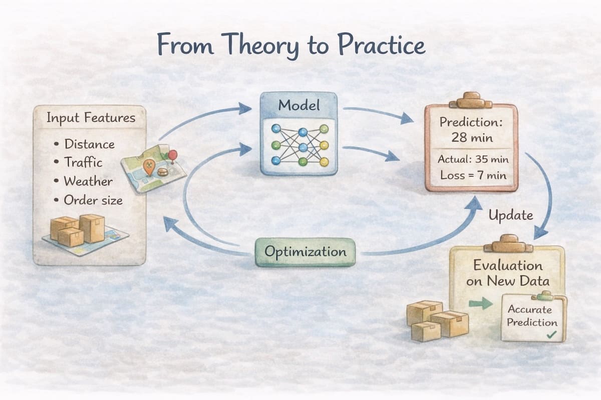
From Theory to Practice

A machine learning model usually follows a similar process:

Define the input features Decide what information will be given to the model.
For example, in a delivery prediction system, this could include distance, traffic level, weather, and order size.
Choose a model (hypothesis function)
This defines how inputs are transformed into predictions.
Select a loss function The loss function determines how prediction errors are measured.
Train the model through optimisation The optimisation process adjusts model parameters to reduce the loss.
Evaluate generalisation Ensure the model performs well on new data and avoids problems like high bias or high variance.

Although modern machine learning systems can involve complex algorithms and large datasets, they all rely on the same core ideas introduced in this chapter. Understanding these fundamentals makes it easier to reason about how models learn and why they sometimes fail.

🧾 Summary

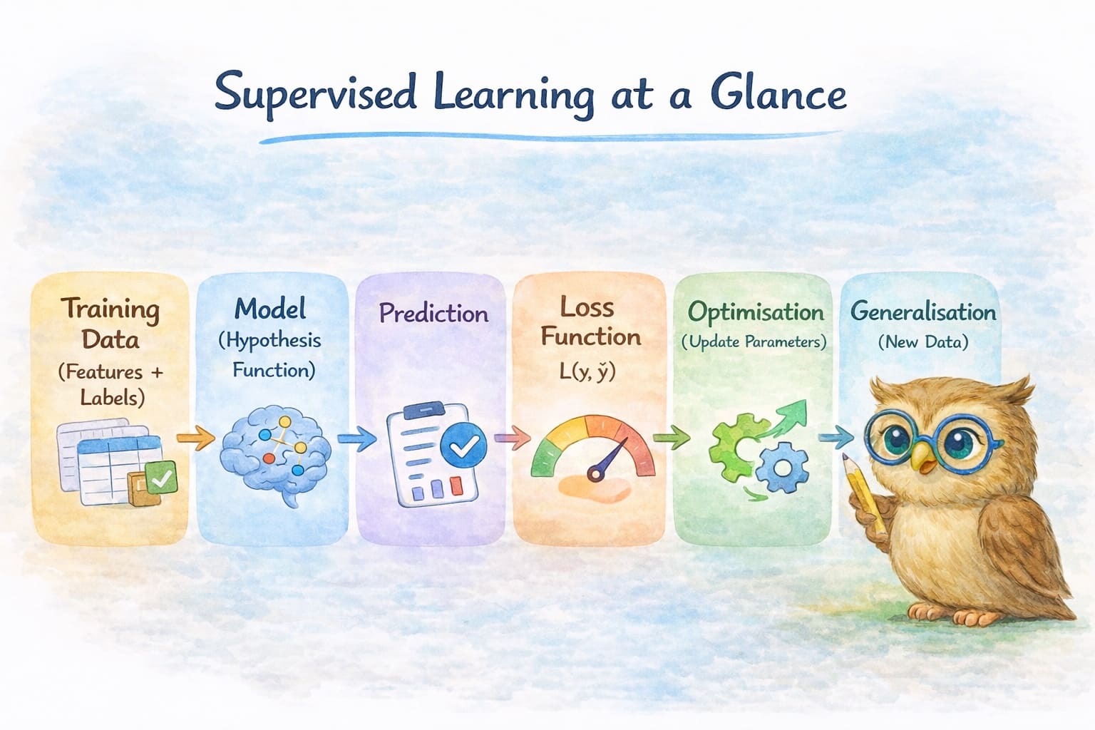
Supervised learning can be understood as a simple but powerful process.

A model represents a simple math function that maps inputs to predictions.
A loss function measures how wrong those predictions are.
An optimisation process adjusts the model parameters to reduce that error.

However, minimising loss alone does not guarantee perfect predictions.
A model may still make mistakes if it is too simple (high bias) or too complex (high variance).

The goal of a good machine learning system is therefore not just to reduce error, but to learn patterns that generalise well to new, unseen data.

Understanding these foundations—hypothesis functions, loss functions, optimisation, and the bias–variance trade-off—gives us the tools to understand how supervised learning algorithms work.

Summary – Voice Recording

Conclusion

This chapter has been quite long, but Tensor Owl wanted to complete the foundational ideas before moving directly to algorithms. We explored what supervised learning really means, how training data provides both inputs and known outputs, and how models learn patterns from these examples. Along the way, we also examined the key building blocks of supervised learning — hypothesis functions, loss functions, optimisation, and the bias–variance trade-off.
With these foundations in place, we are now ready to move forward.

In the next chapter, we will explore our first supervised learning algorithm — Linear Regression — and see how these principles come together to learn from data.