A Question About the Future
In Chapter 3, Tensor Owl  discovered how supervised learning allows a machine to learn from past examples of input and output.
But learning patterns is only the beginning. The real power of that learning appears when the machine starts using those old patterns to estimate what may happen next.
One evening, Tensor Owl returned to his forest home, but something felt different. A large tree near his nest had been cut down by humans. Several birds had lost their homes, and the forest felt quieter than before.
Sitting on a branch, Tensor Owl began to wonder. If trees continue to disappear like this, what will the future look like? And if the human population keeps growing while forests shrink, how long can life on Earth continue in balance?

Instead of simply guessing, Tensor Owl decided to study the past. He began collecting historical data to see whether the old numbers were pointing in some pattern — and whether that pattern could help predict the future.
Once the data was in front of him, the next question was simple: were these numbers moving in some understandable direction? One of the simplest tools machines use to find such a direction is
What is Linear Regression
Picture this: you have decades of data on global forest area, and you plot it on a graph to see which direction these numbers seem to be moving.
Global Forest Area (1950 → 2020): UN FAO & Historical Research Data
| Year | Forest Area (Million Hectares) |
|---|---|
| 1950 | ~4900 |
| 1960 | ~4700 |
| 1970 | ~4550 |
| 1980 | ~4400 |
| 1990 | 4280 |
| 2000 | 4150 |
| 2010 | 4060 |
| 2020 | 4060 |
When we plot these values as coordinates — Year on the x-axis and Forest Area on the y-axis — we get a scatter plot like this:
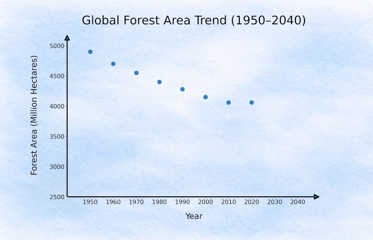
If we observe these points closely, they show a general downward movement over time. Now imagine drawing one straight line through the middle of this downward trend.
It may not pass through every point, but it stays close enough to capture the overall direction hidden inside the data.
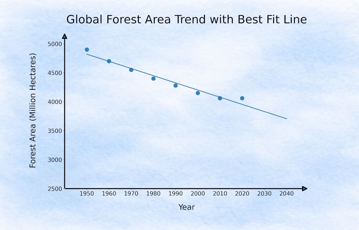
For each actual point on the graph, the line gives its own predicted point. Since the line does not pass through every actual point, there is always a small gap between the two.
Linear Regression tries to find a line that stays as close as possible to all the points. This small gap between the actual value and the predicted value is called a residual error.
Residual Error
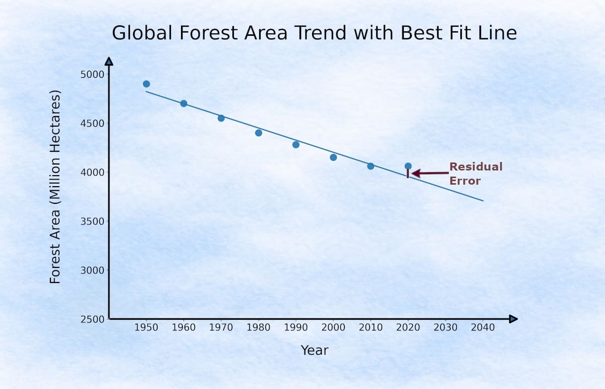
A residual error is simply the difference between the actual value (y) and the predicted value (ŷ). It tells us how far the real data point is from the machine’s current prediction line.
Of course, many different straight lines can be drawn here. So how do we decide which one the machine should choose?
For each line, we measure the gap between the actual points and the predicted points. Instead of simply adding these errors, we square them to avoid positive and negative values canceling each other.
The
Hypothesis
In childhood, Tensor Owl had the same route to school every day. As the bus moved from the crowded city roads toward the outer areas, he would sit by the window and quietly count the trees along the way.
He noticed that as the bus moved farther away from the city centre, the number of trees usually increased. But he also noticed something else — year by year, even those trees were becoming fewer. The city was slowly stretching outward, and wherever it stretched, trees disappeared.
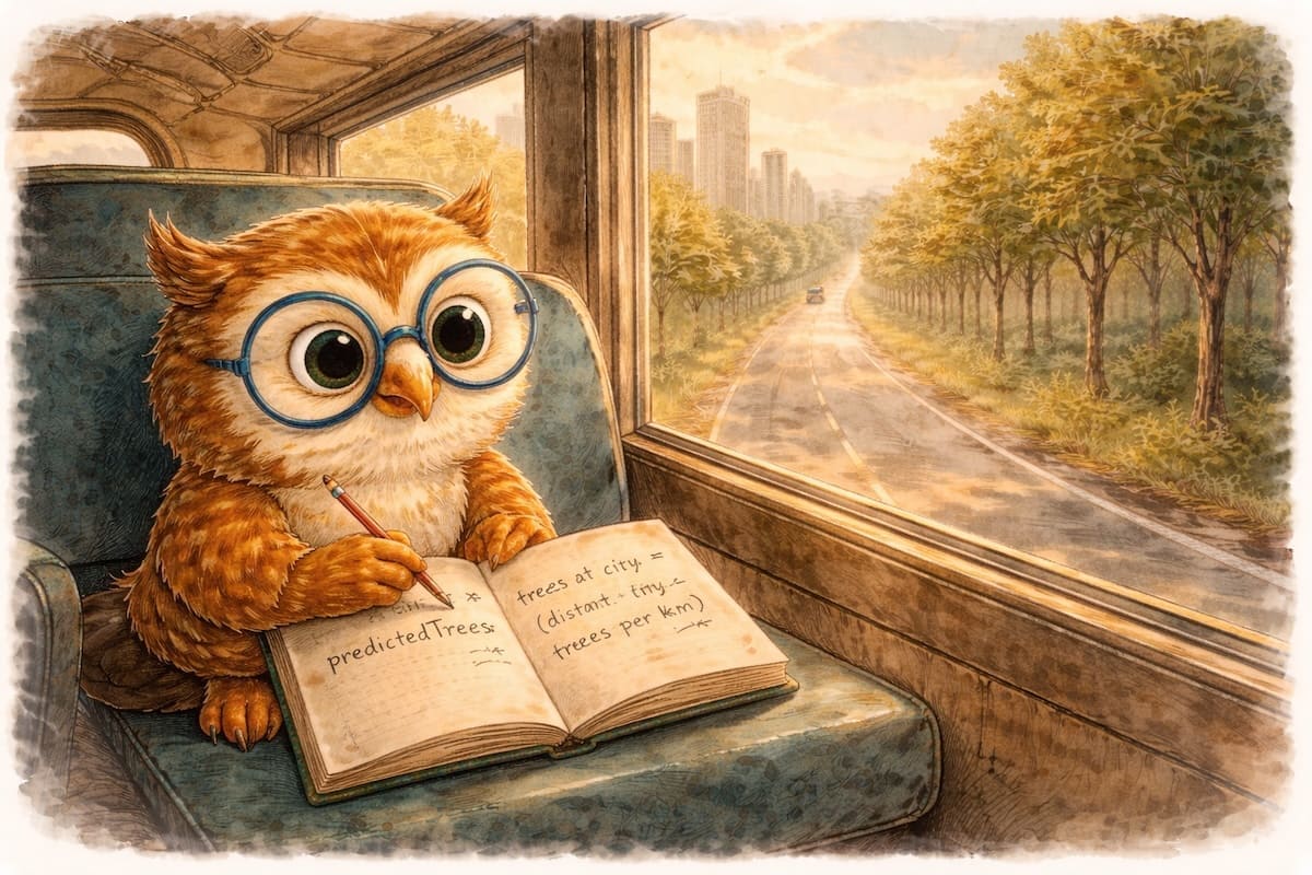
One afternoon, he opened his notebook and tried to express this observation as one simple rule:
predictedTrees = trees at city + (distance from city centre × trees per km)
Without realizing it, Tensor Owl was describing a simple linear relationship. What he had written in his notebook was really the same as the familiar straight-line equation from mathematics:
It was the same simple idea — a straight line showing how one value changes when another value changes.
In machine learning, this same idea is written as a function called the
In our forest example, the machine is trying to learn this same straight-line relationship between year and forest area.
 x — Input Feature:
The value we provide to the model. In this forest study, x is the year.
x — Input Feature:
The value we provide to the model. In this forest study, x is the year.
ŷ — Predicted Output:
The value the model predicts. Here, it is the predicted forest area for a given year.
θ₁ — Slope:
The rate at which the output changes as the input increases. It tells us how much the forest area is rising or falling with each passing year.
θ₀ — Intercept:
The starting value when the input is zero — the point from which the machine begins drawing its prediction line.
Together, θ₀ and θ₁ are called the parameters of the model. A child observes them from experience. A machine learns them from data.
We now have a hypothesis — a line described by θ₀ and θ₁. But there are infinitely many possible lines we could draw through the data. How does the model decide which one is best?
To answer that, the machine needs a formal way to measure its total prediction mistake — and this leads us to the Cost Function.
Cost Function
Every possible line gives its own set of predictions, and each prediction contains some residual error. The cost function gathers all these errors together and produces one single number — a measure of how wrong the current line is across the full dataset.
To measure this properly, we take the difference between actual and predicted values for every point, square those differences, and then combine them into one total error.
The machine now needs one simple way to judge how good or how bad this current line really is.
yᵢ — The actual value for the i-th data point.
ŷᵢ — The predicted value produced by the current line for the same point.
(ŷᵢ − yᵢ)² — The squared residual error for that point.
Squaring removes negative signs and penalises larger errors more heavily than smaller ones.
Σ — We sum these squared errors across all data points.
m — The total number of data points in the dataset.
1/2m — Dividing by m gives the average error.
The factor of ½ is a small mathematical convenience —
it simplifies the calculation in the next step without changing the result.
J(θ) — The final cost value.
A high J(θ) means the line fits poorly. A low J(θ) means the line fits well.
The goal is simple: find θ₀ and θ₁ that make J(θ) as small as possible.
Quick Machine Trial
Before moving ahead, let us watch the model test one possible line on a very small dataset. Suppose Tensor Owl collected only three decades of simplified forest data:
| Decade Index (x) | Actual Forest Area (y) |
|---|---|
| 0 (2000) | 10 |
| 1 (2010) | 8 |
| 2 (2020) | 6 |
To keep the arithmetic simple, let us measure the passing decades as 0, 1, and 2.
Step 1: Hypothesis
Now imagine the machine randomly starts with this hypothesis:
hθ(x) = 12 − x
This means for now the machine has chosen:
θ₀ = 12 and θ₁ = -1
So:
when the decade index increases by 1, the predicted forest area decreases by 1,
and at x = 0 the line begins from 12.
| x | Actual y | Predicted hθ(x) = 12 - x |
|---|---|---|
| 0 | 10 | 12 |
| 1 | 8 | 11 |
| 2 | 6 | 10 |
So each point has some residual error.
Step 2: Residual Errors
| x | Actual y | Predicted ŷ | Error (ŷ - y) |
|---|---|---|---|
| 0 | 10 | 12 | 2 |
| 1 | 8 | 11 | 3 |
| 2 | 6 | 10 | 4 |
Step 3: Square and Sum the Errors
| Error | Squared Error |
|---|---|
| 2 | 4 |
| 3 | 9 |
| 4 | 16 |
Step 4: Compute Cost
So this current line gives a cost of 4.83. The machine now understands that this line is still carrying noticeable error, so it must adjust θ₀ and θ₁ to bring the cost down. And this intelligent adjustment process is called Gradient Descent.
Gradient Descent
In the previous example, the machine tested one line and got a cost of 4.83. This means the line still carries noticeable error.
Now the natural question is:
Do we need to try every possible combination of θ₀ and θ₁ to find the best line?
That would be slow and impractical — there are infinitely many lines.
So the model follows a smarter path. Instead of checking every line, it starts from one random line and keeps adjusting it only in the direction where the cost begins to reduce.
This gradual step-by-step movement toward lower error is called
How Cost Changes as Slope Changes
Let’s simplify the problem for a moment. Assume the intercept is zero and fixed, so the line passes through the origin. Now the cost depends on just one parameter — the slope.
As we change the slope, the predicted points move closer to or farther from the actual points:
When the line is far from the actual values, the predicted points are far away, so the error is large and the cost is high.
As the line gets closer to the actual values, the predictions improve, so the error reduces and the cost decreases.
At the best fit, the predicted points are closest to the actual values, so the error is minimum and the cost is lowest.
If we move past this point, the predictions start getting worse again, so the error increases and the cost rises.
Think of it like adjusting a line by hand — as you rotate it, you see the points getting closer, then perfectly aligned, and then drifting away again.
If you observe the cost chart, the
At this point:
The predicted line is closest to all actual data points.
The total residual error is minimum.
The model has found the best possible fit for the current data.
So instead of trying every line manually, the model simply needs to move toward this lowest point on the cost curve.
And the method used to move toward this minimum cost is called
“How does it know where the next step should go?”
Finding the Direction of Improvement
Now we know that the best fit line lies at the lowest point of the cost curve. But the model still does not know where that point is.
Once the model calculates the cost for its current slope value, a natural question comes to mind:
Let us suppose the model is currently at
- Should it slightly increase the slope to 0.9?
- Or should it decrease the slope to 0.7?
To make this decision, the model checks how the cost graph is behaving at the current point.
Let us focus on the point where
This tiny touching line tells the machine one practical thing: if the slope changes just a little, will the cost begin to rise or begin to fall?:
- if a line rises as we move from left to right, its slope is positive.
- if a line falls as we move from left to right, its slope is negative.
Now look at the touching line at θ₁ = 0.8. It falls toward the right, so the slope is negative.
That means if we increase θ₁ slightly, the cost will begin to decrease.
So the model understands that moving right will improve the current line.
Similarly, at θ₁ = 2.2, the touching line rises toward the right, so the slope is positive.
That means moving further right would increase the cost, so the model should move left instead.
And near θ₁ = 1.5, the touching line becomes almost flat.
That tells the model it is very close to the minimum cost point.
This local slope is calculated mathematically by measuring how much the Cost Function changes for a very tiny change in
So the derivative tells the model one simple thing: which direction will reduce the current error.
But knowing only the direction is still not enough. The model must also decide:
how big should the next move be?
- Should it move just a little?
- Or should it take a large jump?
This is controlled by another important value called the Learning Rate.
Learning Rate
The derivative tells the model which direction will reduce the error. Now the model must decide how big that next move should be.
- A very small move makes learning slow.
- A very large move can jump past the minimum cost point.
So the model updates the slope using a controlled step size called the
Now the model knows both — which direction to move and how large that move should be. So it is finally ready to update the current slope.
Gradient Descent Update Rule
The model now has everything it needs for one intelligent correction:
- the Derivative tells which direction lowers the cost,
- the Learning Rate tells how big the next move should be.
By combining both, the model updates the current slope using:
In simple words, the machine does this:
new θ₁ = current θ₁ - (Learning Rate × Cost Derivative)
Now notice the minus sign carefully.
The model always wants to move toward lower cost. So it subtracts the derivative value automatically:
- if the derivative is positive, subtraction makes
θ₁ smaller, so the model moves left. - if the derivative is negative, subtraction makes
θ₁ larger, so the model moves right.
In both cases, the minus sign pushes the model toward the side where the cost begins to fall.
For example, if the current slope is 0.8 and the derivative tells the machine to move right, the next update may push θ₁ a little closer to 0.9, then 1.0, and gradually toward the minimum.
So after every update, the regression line becomes a little better than before.
The model keeps repeating this same correction again and again until the cost can no longer reduce significantly.
At that point, it has reached the best possible fit.
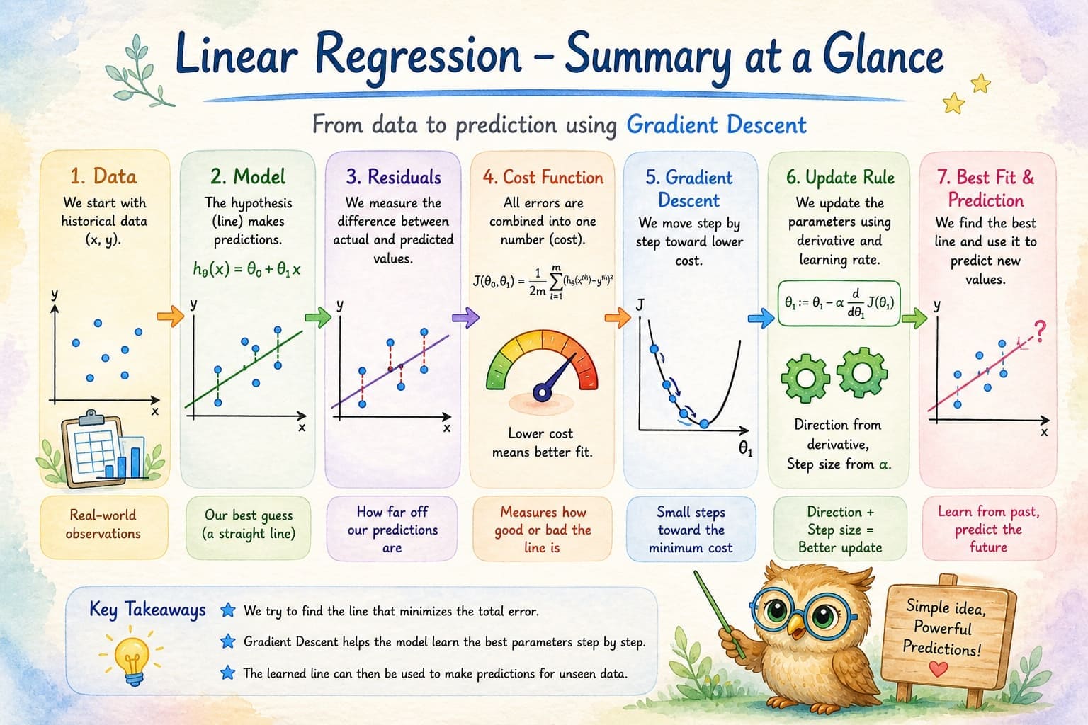
🧾 Summary
Linear Regression is one of the simplest ways a machine learns to make predictions from past data.
- The
hypothesis is the model’s current guess of the relationship between input and output. - For every data point, the machine compares its predicted value with the actual value and measures the difference, called the
residual error . All these residual errors are combined inside aCost Function , which tells the machine how well or how poorly the current line fits the data. - The machine then improves this line using
Gradient Descent — a step-by-step process that keeps adjusting the model parameters toward lower cost.
To make each adjustment, the machine uses:
- The
Derivative to know which direction reduces the error, and theLearning Rate to decide how large the next move should be. - By repeating these small corrections again and again, the model gradually reaches the
best fit line . Once this line is learned from historical data, the machine can use it to make sensible predictions for future values it has not seen before.
Summary – Voice Recording
Conclusion
This chapter took us inside the quiet depth of machine prediction.
Tensor Owl began with a simple concern — if forests continue to disappear, can old records help reveal where this path leads?
Through Linear Regression, we discovered that the machine does not guess blindly. It studies the past, measures its mistakes, and keeps correcting itself until a meaningful pattern begins to appear.
By the end, Tensor Owl understood that every prediction line is built from the past — old numbers quietly helping the machine estimate what may come next.
Tensor Owl also came to a silent realisation: humans often see the forest as land, timber, or expansion, but rarely as a living neighbourhood shared by countless beings whose homes vanish without a voice.
In the next chapter, we will take this same prediction idea one step further and explore how machines build stronger regression models when many different input features influence the final outcome together.
Code Sample
For readers who wish to see how this entire learning process looks in actual Python code, a small companion implementation using the same forest dataset is available on GitHub:
View Linear Regression Python Implementation on GitHub
🔎 Recap & Reflection
A forest department already has a model that predicts the exact number of hectares likely to remain after each decade. Now another officer asks: 'Will this forest region become environmentally dangerous within 20 years — Yes or No?' Can the same Linear Regression model answer this new question correctly?
A model learns to predict forest area using only the year as input. The hypothesis is: predicted_area = θ₀ + θ₁ × year. After training, θ₀ = 4900 and θ₁ = -2.5. What does θ₁ = -2.5 tell you about the relationship between year and forest area?
Two prediction lines are tested on the same forest dataset. Line A leaves residual errors: 2, 2, 2, 2 Line B leaves residual errors: 0, 0, 0, 8 Which line is more likely to be preferred by the Cost Function?
The machine is standing at a point on the cost curve where moving slightly to the right makes the cost smaller. But instead of moving a little, it jumps too far to the right and lands on a higher point again. What most likely caused this?
During gradient descent, the model calculates the derivative of the cost function at θ₁ = 0.5 and finds it to be negative (-0.8). According to the gradient descent update rule: θ₁ := θ₁ - α × (derivative) If α = 0.1, which direction will θ₁ move, and why?
A machine learning engineer trains two linear regression models on the same dataset: Model A: Learning rate α = 0.001 (very small) Model B: Learning rate α = 0.5 (very large) What is the most likely difference in their behavior during training?
A regression model makes the following predictions for three forest data points: Point 1: Actual = 4500, Predicted = 4600 (Error = 100) Point 2: Actual = 4200, Predicted = 4200 (Error = 0) Point 3: Actual = 3900, Predicted = 3800 (Error = -100) When calculating the cost function J(θ), why do we square these errors before summing them?
A forest prediction model is trained and reaches a cost value of J(θ) = 0.05. After 100 more training iterations, the cost remains at 0.05 and stops decreasing. The derivative at this point is approximately 0. What does this tell you about the model?
Rate this article
Loading...